Pytorch

Preparations

Windows 11; Pycharm

Cuda的安装与卸载

先查看包的安装情况，然后一个个卸载

dpkg -l |grep cuda
apt-get purge --auto-remove ...

pi cuda-toolkit-11-7-config-common 11.7.99-1 all Common config package for CUDA Toolkit 11.7.
pi cuda-toolkit-11-config-common 11.8.89-1 all Common config package for CUDA Toolkit 11.
pi cuda-toolkit-config-common 12.0.107-1 all Common config package for CUDA Toolkit.

删不掉

dpkg –remove –force-remove-reinstreq cuda-toolkit-11-7-config-common cuda-toolkit-11-config-common cuda-toolkit-config-common

还不行

dpkg –remove libcublas-11-7 libnpp-11-7 libcusparse-11-7

还不行

dpkg –remove libcublas-dev-11-7 libnpp-dev-11-7 libcusparse-dev-11-7

dpkg –remove libcublas-11-7 libnpp-11-7 libcusparse-11-7

dpkg –remove –force-remove-reinstreq cuda-toolkit-11-7-config-common cuda-toolkit-11-config-common cuda-toolkit-config-common

还不行

dpkg –purge –force-remove-reinstreq cuda-toolkit-11-7-config-common cuda-toolkit-11-config-common cuda-toolkit-config-common

解决

sudo apt-get autoremove
sudo apt-get autoclean
sudo apt-get install -f

sudo dpkg –configure -a
sudo apt-get update
sudo apt-get upgrade

Win-Anaconda

Choose the suitable version to download.

Check the version installed.

conda --version

Add the system environment variables.

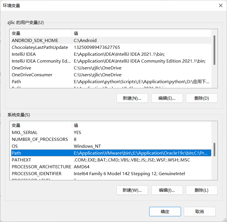
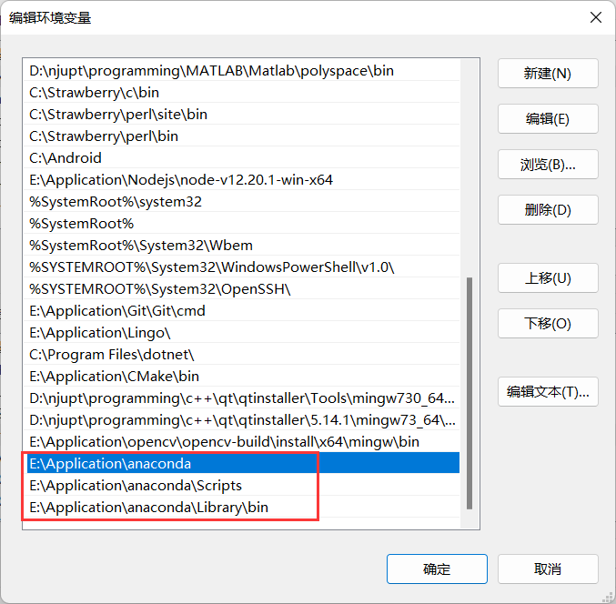
Check the GPU cuda version

nvidia-smi

Win-Pytorch

You can choose official command to download.

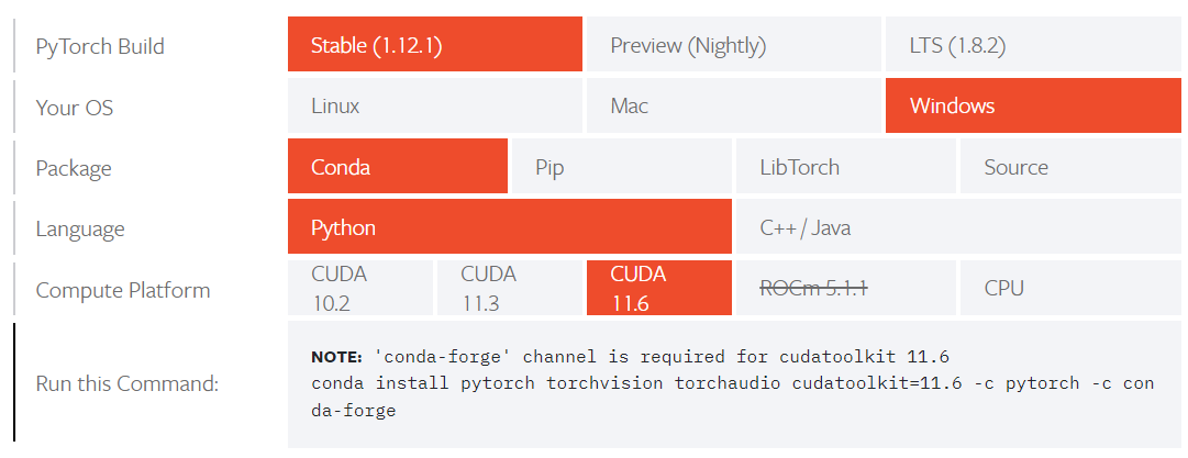
Sometimes your domestic network can’t be connected to the official service. So choose the link of tsinghua’s mirrors.

conda config --add channels https://mirrors.tuna.tsinghua.edu.cn/anaconda/pkgs/free/
conda config --add channels https://mirrors.tuna.tsinghua.edu.cn/anaconda/pkgs/main/
conda config --add channels https://mirrors.tuna.tsinghua.edu.cn/anaconda/cloud/pytorch/
conda config --add channels https://mirrors.tuna.tsinghua.edu.cn/anaconda/cloud/conda-forge/
conda config --add channels https://mirrors.tuna.tsinghua.edu.cn/anaconda/cloud/menpo/
conda config --add channels https://mirrors.tuna.tsinghua.edu.cn/anaconda/cloud/bioconda/
conda config --add channels https://mirrors.tuna.tsinghua.edu.cn/anaconda/cloud/msys2/
conda config --add channels https://mirrors.tuna.tsinghua.edu.cn/anaconda/cloud/peterjc123/
conda config --set show_channel_urls yes

You can check the channels added.

conda config --show

Or change the channels for the initial states.

conda config --remove-key channels

Then start to install.

conda install pytorch torchvision torchaudio cudatoolkit=11.6

Wait for several minutes and check the installation state.

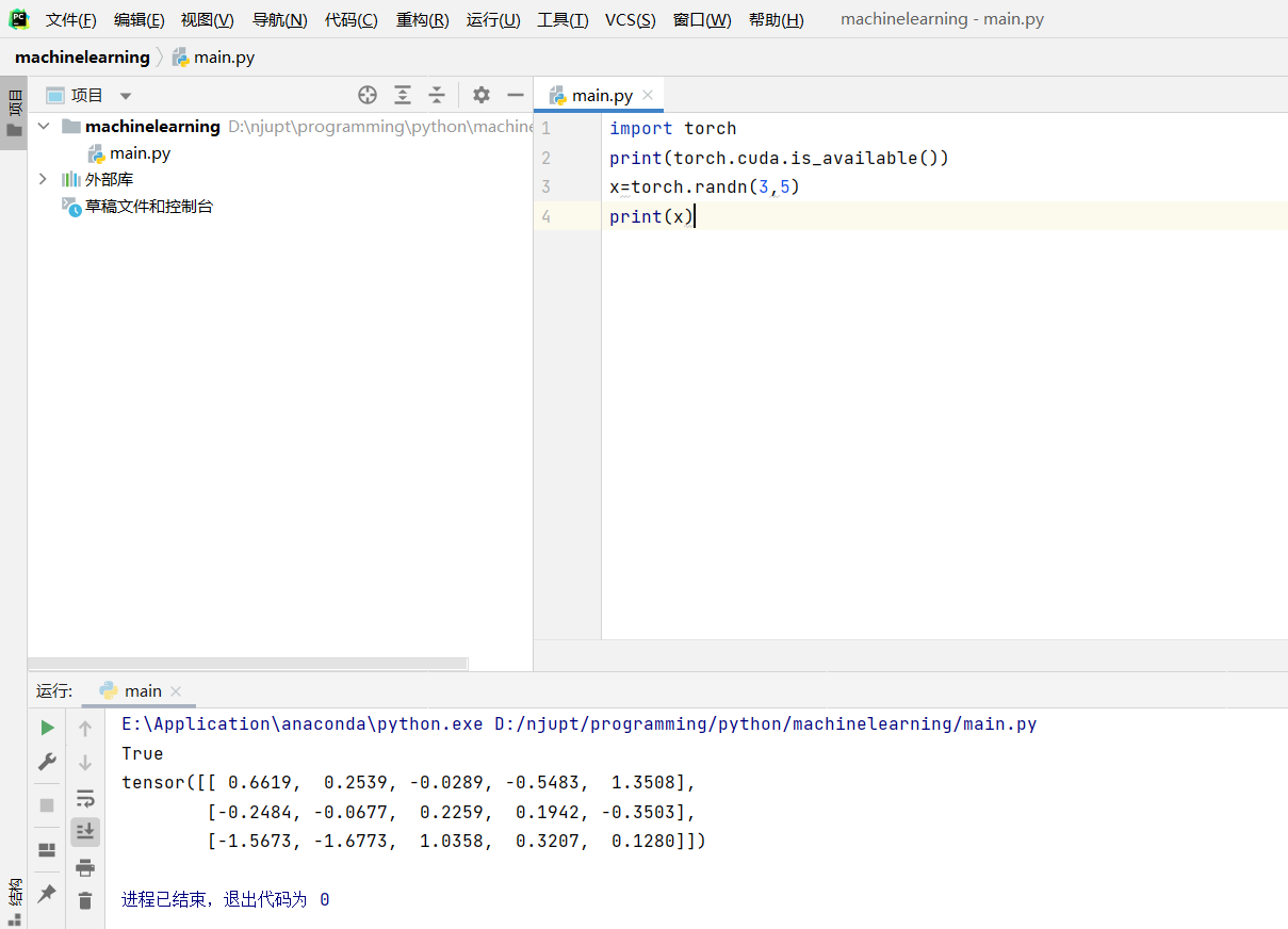
import torch
print(torch.cuda.is_available())
x=torch.randn(3,5)
print(x)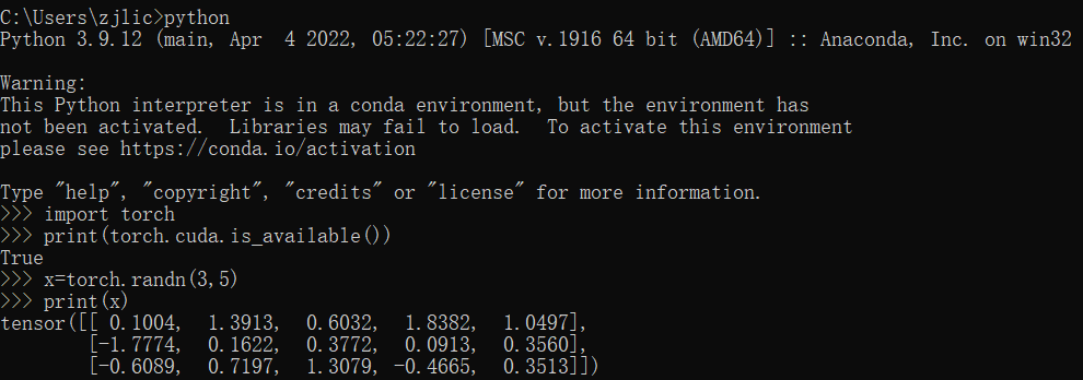

Win-Pycharm

Create one python file and configure the settings (files-settings).

Choose your python interpretation.

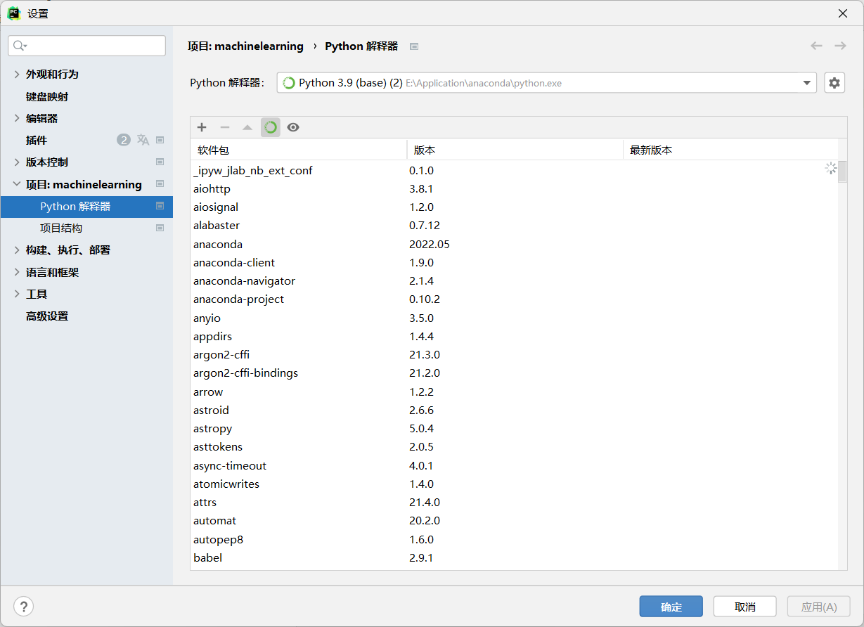
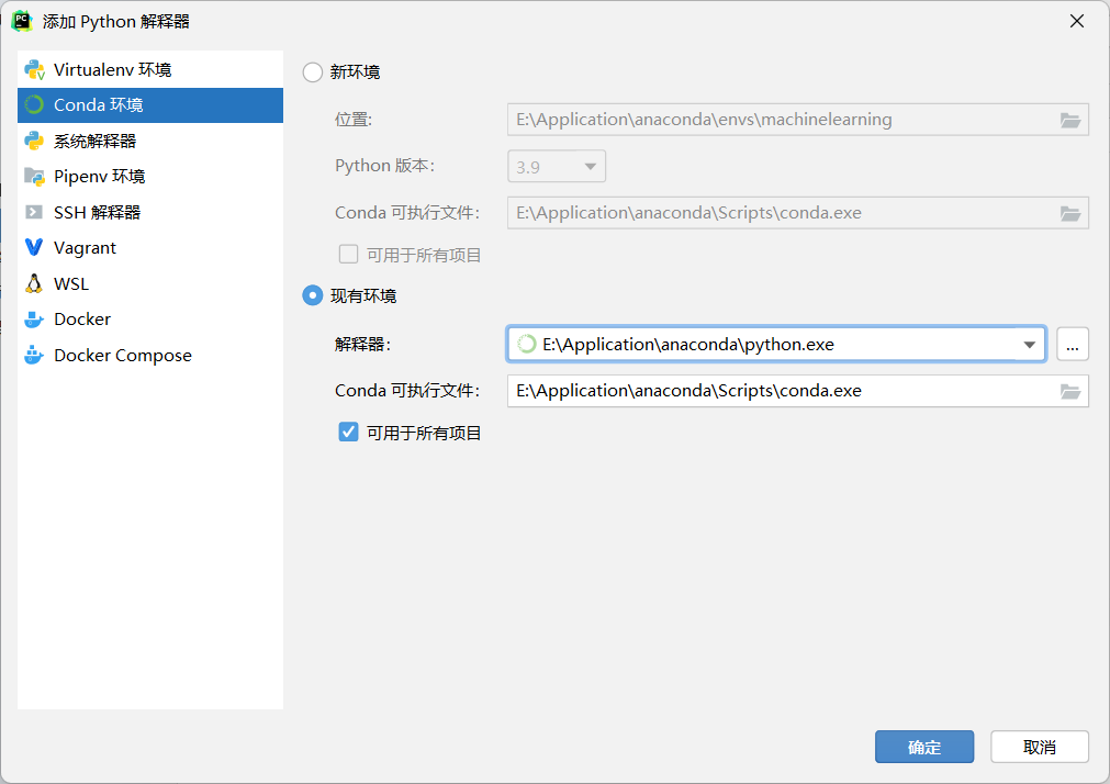
Add the conda environment.

Notice: Because of the difference between the Linux and Windows, Windows can install the pytorch without using virtual environment, so we need to choose the python interpretation at the base environment (Choose the python.exe at the basic catalogue and choose the button suitable for all the projects).

After that, compile the codes checked before.

Practice

import torch					#If we want to use GPU, we need to use ".cuda()"
x=torch.arange(12).cuda()       #create the tensor like vector(initiate from 0)
s=x.reshape(3,4).cuda()         #reshape the dimension(row3line4)
print(s.shape)                  #the attribution of tensor(length of each dimension)
print(s.numel())                #multiple the length of all the dimensions
print(torch.ones((2,3,4)))      #(z,x,y) and all the elements are 1
print(torch.randn(3, 4))        #the elements random from standard normal distribution(SND)
print(torch.tensor([[2, 1, 4, 3], [1, 2, 3, 4], [4, 3, 2, 1]]))#Manual assignment
x = torch.tensor([1.0, 2, 4, 8])
y = torch.tensor([2, 2, 2, 2])
print(torch.exp(x) ** y)        #Exponentiation
X = torch.arange(12, dtype=torch.float32).reshape((3,4))
Y = torch.tensor([[2.0, 1, 4, 3], [1, 2, 3, 4], [4, 3, 2, 1]])
print(torch.cat((X, Y), dim=0)), print(torch.cat((X, Y), dim=1))#dimension0 vertical connection;dimension1 horizontal connection
print(X==Y)                     #judge the element at the same position
#2.1 data operation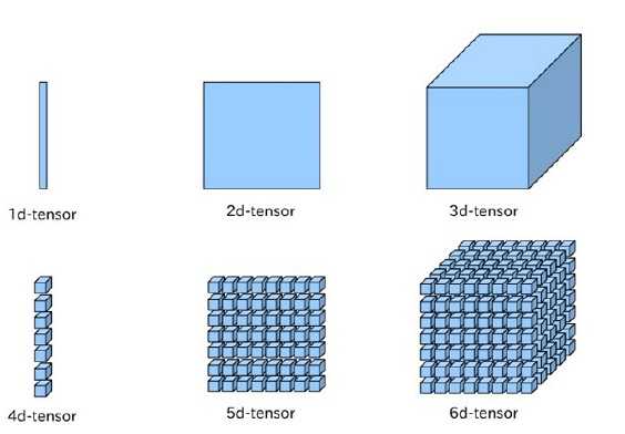

broadcast mechanism

If there is one row in tensor, copy the row; If there is one line in tensor, copy the line.

For example, 3*1 plus 1*2 equals 3*2

index mechanism

X[0:2, :] = 12

0-1 rows and all the lines selected

Save memory

Y[:] = <expression>
X[:] = X + Y
X += Y

Transform

A = X.numpy()
B = torch.tensor(A)
a = torch.tensor([3.5])
a, a.item(), float(a), int(a)#last three variables represent the single value

File operation

import os
import pandas as pd
import torch
os.makedirs(os.path.join('..', 'data'), exist_ok=True) # create the folder "data" at local directory
data_file = os.path.join('..', 'data', 'house_tiny.csv')
with open(data_file, 'w') as f:
    f.write('NumRooms,Alley,Price\n')
    f.write('NA,Pave,127500\n')
    f.write('2,NA,106000\n')
    f.write('4,NA,178100\n')
    f.write('NA,NA,140000\n')
data = pd.read_csv(data_file)
print(data)
inputs, outputs = data.iloc[:, 0:2], data.iloc[:, 2] # the data read from csv needs "iloc" index mechanism
inputs = inputs.fillna(inputs.mean()) # fill the NaN with the mean value of inputs(this will get an error because there is non-numeric value)
inputs = pd.get_dummies(inputs, dummy_na=True) # for the class discrete value, pd will divide the "Pave" and "Nan" into two category and fill with "1" and "0"(transform into numeric value)
X, y = torch.tensor(inputs.values), torch.tensor(outputs.values) # tranform into torch
print(X,y)

High dimension

X = torch.arange(24).reshape(2, 3, 4) # height:2, row:3, line:4

Allocate new memory

B = A.clone() # Allocate new memory with A for B

Dimension reduction

We know that the axis of tensor depends on the order of dimension, such as [2,3,4] represents the height is 2, the row is 3 and the line is 4. So the axis 0 represents height, the axis 1 represents row and 3 represents line.

We use the sum to reduce the dimension. If we set the axis 0, we will kill the dimension 0.

A = torch.arange(20, dtype=torch.float32).reshape(5, 4)
A_sum_axis0 = A.sum(axis=0)
A_sum_axis0, A_sum_axis0.shape
(tensor([40., 45., 50., 55.]), torch.Size([4]))
A.sum(axis=[0, 1]) # SameasA.sum(), the sum of all the elements
sum_A = A.sum(axis=1, keepdims=True) # retain two dimensions to get sum
A.cumsum(axis=0) # to get cumulative sum from row
tensor([[ 0., 1., 2., 3.],
[ 4., 6., 8., 10.],
[12., 15., 18., 21.],
[24., 28., 32., 36.],
[40., 45., 50., 55.]])

Dot product

import torch
x = torch.arange(4, dtype = torch.float32)
y = torch.arange(4, dtype = torch.float32)
print(x*y) # the result is a tensor("Hadamard product" by element at the same position)
print(torch.dot(x, y)) # the result is the sum of tensor(x*y)

# The column dimension of A (length along axis 1) must be the same as the dimension of x (matrix-vector product)
A = torch.arange(20,dtype=torch.float32).reshape(5, 4).cuda()
x = torch.arange(4,dtype=torch.float32).cuda()
print(x,"\n",A,"\n",torch.mv(A, x).cuda())
# tensor([ 14.,  38.,  62.,  86., 110.], device='cuda:0') cuda can't use int and long

Matrix product

print("\nmm(A, B)=",torch.mm(A, B).cuda(),'\n')

Norm

Vector norm has three attributions f(ax) =∣a∣f(x) and Triangle Inequality and non-negative

The sum of squares transformation is not a definition of vector norm because it does not satisfy some basic properties of norm, such as the triangle inequality and positive-definiteness. However, it is still a commonly used method for vector transformation, which is often applied in machine learning and deep learning tasks, such as feature extraction and representation learning.

L2 norm is the square root of the sum of squares of vector elements. (Euclidean distance)

u = torch.tensor([3.0, -4.0])
torch.norm(u)

L1 norm is represented as the sum of absolute values of vector elements.

torch.abs(u).sum()

Lp norm is more generalized.
$$
||x||_p=(\sum^{n}_{i=1}|x_i|^p)^{\frac{1}{p}}
$$
Frobenius norm is the L2 norm of the matrix.
$$
||x||_F=\sqrt{(\sum^{m}_{i=1}\sum^{n}_{j=1}x_{ij}^2)}
$$

torch.norm(torch.ones((4, 9)))
tensor(6.)

Differentiation

%matplotlib inline
import numpy as np
import matplotlib.pyplot as plt# 导入matplotlib库
def f(x):
	return 3 * x ** 2 - 4 * x
def numerical_lim(f, x, h):
	return (f(x + h) - f(x)) / h
h = 0.1
for i in range(5):
	print(f'h={h:.5f}, numerical limit={numerical_lim(f, 1, h):.5f}') #rounding to 5 decimal places with f-string (float)
	h *= 0.1
    
#h=0.10000, numerical limit=2.30000
#h=0.01000, numerical limit=2.03000
#h=0.00100, numerical limit=2.00300
#h=0.00010, numerical limit=2.00030
#h=0.00001, numerical limit=2.00003

# 定义x的取值范围 在[-5, 5]这个区间中生成长度为100的等差数列，生成的每个数值都被保存在x中
x = np.linspace(-5, 5, 100)

plt.plot(x, f(x), label='f(x)')# 绘图
# 设置xy轴标签
plt.xlabel('x')
plt.ylabel('f(x)')
# 展示标题
plt.title('Function f(x)')
# 展示图例
plt.legend()
# 展示图像
plt.show()

#  设置切点
x1 = 1
y1 = f(x1)
# 设置斜率
slope = 2
# 根据切点和斜率写出切线
y2 = y1 + slope * (x - x1)

plt.plot(x, f(x))
plt.plot(x, y2)
plt.xlabel('x')
plt.ylabel('y')
plt.title('Function f(x) and its tangent at x=1')
plt.legend(['Function f(x)', 'Tangent line at x=1'])#可以通过设置 label 参数为每个数据系列指定一个标签，然后使用 legend 函数在图表中显示这些标签。
plt.show()

Plot with PyCharm

Based on pycharm and anaconda, there is some steps:

1. Set the step and range of x
2. Define the function
3. Plot the graph with the label # plt.plot(x, f(x), label=’f(x)’)
4. Set the label of xy axis
5. Set the title
6. Show the label # plt.legend() or plt.legend([' ',' '])
7. Show the graph # plt.show()

Gradient

The set of partial derivative of a multivariable function with respect to each of its variables.
$$
\begin{gathered}
\nabla f(x_1, x_2, \ldots, x_n) = \begin{bmatrix}\frac{\partial f(x)}{\partial x_1} \frac{\partial f(x)}{\partial x_2} ,\ldots,\frac{\partial f(x)}{\partial x_n}\end{bmatrix}^T\cr
\nabla_xAx=A^T\cr
\nabla_xx^TA=A\cr
\nabla_xx^TAx=(A+A^T)x\cr
\nabla_x||x||^2=\nabla_xx^Tx=2x\cr
\nabla||A||^2_F=2A
\end{gathered}
$$

We can understand the formula by using quadratic forms in linear algebra.

Gradient tracking

import torch
x = torch.arange(4.0)
# tensor([0., 1., 2., 3.])
x.requires_grad_(True) # 等价于x=torch.arange(4.0,requires_grad=True)
x.grad # 默认值是None
y = 2 * torch.dot(x, x)
tensor(28., grad_fn=<MulBackward0>)